Introduction
Survival analysis can be used to analyze the time it takes for some event of interest to occur. In a medical context the event of interest is often death. The expression “death analysis” sounds rather gloomy so people said “survival analysis”, which sounds much more positive.
If we look at cancer studies, there are three main types of event that we’re interested in, namely
- Relapse – The time before someone’s health deteriorates after a temporary improvement
- Progression – The time before someone’s health state changes (for better or worse)
- Death – The time before someone dies
Because any study using survival analysis has a clear beginning and end, it may very well be that for some patients the event of interest has not occurred within the study time period, but it might have if the study ran longer. This introduces uncertainty for these patients and means that the repeated measurements for these patients are censored. Basically, data collection for these patients is incomplete. Survival analysis was particularly designed to deal with such incomplete data.
There are two types of probability being modeled in survival analysis:
- Survival probability – The probability that a patient is still alive after a certain time period, after being diagnosed with the disease. This probability is defined by \(S(t)\), i.e., the survival function. For example, \(S(200) = 0.7\) means that after 200 days the probability of survival for this patient is 70%.
- Hazard probability – This is simply one minus the survival probability, \(1 – S(t)\), or the probability that the patient is dead after a certain time period.
The survival function \(S(t)\) can be estimated from so-called lifetime data using the Kaplan-Meier estimator. It works like this:
Let’s assume you have a study starting at time \(T_0\) and ending at time \(T_N\). Let’s also assume that at time \(T_0\) and \(T_1\) every patient is still alive, but at \(T_2\) 24% of patients has died. Based on this information we can say that from \(T_1\) to \(T_2\) the probability of dying is 0.24. If at \(T_3\) another 15% of the remaining patients has died, this means that the probability of dying between \(T_2\) and \(T_3\) is 0.15. If we want to calculate the overall probability of a patient dying between \(T_0\) and \(T_3\) we need to multiply the probabilities of each time interval as follows:
- From \(T_0\) to \(T_1\) = 0.0
- From \(T_1\) to \(T_2\) = 0.24
- From \(T_2\) to \(T_3\) = 0.15
For a total probability of 0.0 x 0.24 x 0.15 = 0.036, or 3.6%. The formula for calculating this for any timepoint \(t\) is:
\[ S(t) = \prod_{t_i < t} \frac{n_i – d_i}{n_i} \]
where \(n_i\) is the number of patients still alive just before \(t_i\) and \(d_i\) is the number of events (deaths) that have occurred at \(t_i\).
Example data
The example data used in this post is a lung cancer dataset which can be downloaded here. This dataset contains the following columns:
- inst – Institution code
- time – Survival time in days
- status – Censoring status where 1 = censored and 2 = dead
- age = Age in years
- sex = Sex where 1 = male and 2 = female
- …
Creating Kaplan-Meier plots
import pandas as pd
import numpy as np
import matplotlib.pyplot as plt

from lifelines import KaplanMeierFitter

df = pd.read_csv('lung.csv')

# add column mapping status to mortality
df.loc[df.status==1, 'dead'] = 0
df.loc[df.status==2, 'dead'] = 1
df.head()
which produces the output:
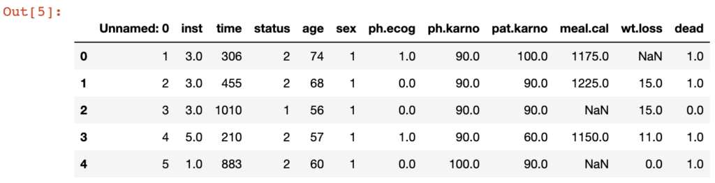
As you can see, we added a binary column “dead” which is required for the Kaplan-Meier fitter, as shown in the code below:
kmf = KaplanMeierFitter()
kmf.fit(durations=df.time, event_observed=df.dead)
kmf.event_tabl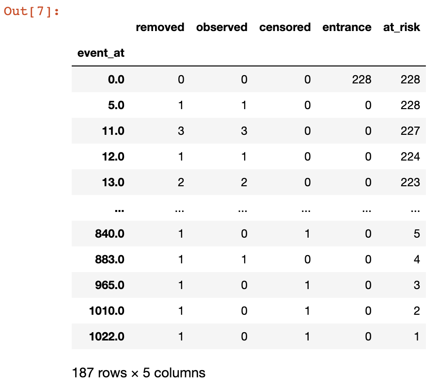
How should we interpret the different columns? First of all, the event_at column shows the number of days that have passed, i.e., the time points, when patients were measured or observed. So you have a group of patients at \(T_0\), i.e., zero days. Then at different time points (ideally equally-spaced but this is not always possible) the group is observed again and you check how many people are still alive and participating, alive but no longer participating (censored) or dead.
If new patients come into the study they are added to the entrance column, thereby increasing the at_risk column as well.
If patients die during the study, they are added to the observed column, and subtracted from the at_risk column. If they are alive but step out of the study they are added to the censored column and subtracted from the at_risk column. If they are still alive when the study ends, they are also added to the censored column. If patients are either dead or censored they are added to the removed column, so removed = observed + censored.
With the information from the table above we can easily calculate the survival probabilities at each time point. For example, at \(T_0\) which corresponds to the first row in the table, we see that there have been 0 observed deaths and 228 patients alive (but at risk). So the survival probability at zero days is calculated as
event_at_0 = kmf.event_tabl.iloc[0,:]
surv_for_0 = (event_at_0.at_risk - event_at_0.observed) / event_at_0.at_risk
or
\[S(0) = \frac{228 – 0}{228} = 1\]
Similarly, the survival probability at 5 days (2nd row in table) is calculated as
event_at_5 = kmf.event_tabl.iloc[1,:]
surv_for_5 = (event_at_5.at_risk - event_at_5.observed) / event_at_5.at_risk
or
\[S(5) = \frac{228 – 1}{228} = 0.9956\]
and survival probability at 11 days (3rd row in table) is calculated as
event_at_11 = kmf.event_tabl.iloc[2,:]
surv_for_11 = (event_at_11.at_risk - event_at_11.observed) / event_at_11.at_risk
or
\[S(11) = \frac{227 – 3}{227} = 0.9867\]
To obtain the survival probability after 11 days we need to multiply the above probabilities
\[S(11)^* = S(0) \times S(5) \times S(11) = 1 \times 0.9956 \times 0.9867 = 0.9823\]
Obviously, the above-mentioned KaplanMeierEstimator can calculate these cumulative probabilities very easily as follows:
kmf.predict(11)
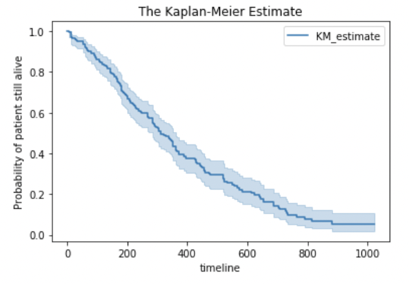
>> 0.9823Similarly, you can use the KaplanMeierEstimator to create a curve:
kmf.plot()
plt.title('The Kaplan-Meier Estimate')
plt.ylabel('Probability of patient still being alive')
plt.show()